Homework 1, Parallelized Dynamics

Chris Rackauckas

September 15th, 2020

Due October 1st, 2020 at midnight EST.

Homework 1 is a chance to get some experience implementing discrete dynamical systems techniques in a way that is parallelized, and a time to understand the fundamental behavior of the bottleneck algorithms in scientific computing.

Please email the results to crackauc@mit.edu titled "Homework 1: (Your Name)".

Problem 1: A Ton of New Facts on Newton

In this problem we will look into Newton's method. Newton's method is the dynamical system defined by the update process:

\[ x_{n+1} = x_n - \left(\frac{dg}{dx}(x_n)\right)^{-1} g(x_n) \]

For these problems, assume that $\frac{dg}{dx}$ is non-singular.

Part 1

Show that if $x^\ast$ is a steady state of the equation, then $g(x^\ast) = 0$.

Part 2

Take a look at the Quasi-Newton approximation:

\[ x_{n+1} = x_n - \left(\frac{dg}{dx}(x_0)\right)^{-1} g(x_n) \]

for some fixed $x_0$. Derive the stability of the Quasi-Newton approximation in the form of a matrix whose eigenvalues need to be constrained. Use this to argue that if $x_0$ is sufficiently close to $x^\ast$ then the steady state is a stable (attracting) steady state.

Part 3

Relaxed Quasi-Newton is the method:

\[ x_{n+1} = x_n - \alpha \left(\frac{dg}{dx}(x_0)\right)^{-1} g(x_n) \]

Argue that for some sufficiently small $\alpha$ that the Quasi-Newton iterations will be stable if the eigenvalues of $(\left(\frac{dg}{dx}(x_0)\right)^{-1} g(x_n))^\prime$ are all positive for every $x$.

(Technically, these assumptions can be greatly relaxed, but weird cases arise. When $x \in \mathbb{C}$, this holds except on some set of Lebesgue measure zero. Feel free to explore this.)

Part 4

Fixed point iteration is the dynamical system

\[ x_{n+1} = g(x_n) \]

which converges to $g(x)=x$.

What is a small change to the dynamical system that could be done such that $g(x)=0$ is the steady state?
How can you change the $\left(\frac{dg}{dx}(x_0)\right)^{-1}$ term from the Quasi-Newton iteration to get a method equivalent to fixed point iteration? What does this imply about the difference in stability between Quasi-Newton and fixed point iteration if $\frac{dg}{dx}$ has large eigenvalues?

Problem 2: The Root of all Problems

In this problem we will practice writing fast and type-generic Julia code by producing an algorithm that will compute the quantile of any probability distribution.

Part 1

Many problems can be interpreted as a rootfinding problem. For example, let's take a look at a problem in statistics. Let $X$ be a random variable with a cumulative distribution function (CDF) of $cdf(x)$. Recall that the CDF is a monotonically increasing function in $[0,1]$ which is the total probability of $X < x$. The $y$th quantile of $X$ is the value $x$ at with $X$ has a y% chance of being less than $x$. Interpret the problem of computing an arbitrary quantile $y$ as a rootfinding problem, and use Newton's method to write an algorithm for computing $x$.

(Hint: Recall that $cdf^{\prime}(x) = pdf(x)$, the probability distribution function.)

Part 2

Use the types from Distributions.jl to write a function my_quantile(y,d) which uses multiple dispatch to compute the $y$th quantile for any UnivariateDistribution d from Distributions.jl. Test your function on Gamma(5, 1), Normal(0, 1), and Beta(2, 4) against the Distributions.quantile function built into the library.

(Hint: Have a keyword argument for $x_0$, and let its default be the mean or median of the distribution.)

Problem 3: Bifurcating Data for Parallelism

In this problem we will write code for efficient generation of the bifurcation diagram of the logistic equation.

Part 1

The logistic equation is the dynamical system given by the update relation:

\[ x_{n+1} = rx_n (1-x_n) \]

where $r$ is some parameter. Write a function which iterates the equation from $x_0 = 0.25$ enough times to be sufficiently close to its long-term behavior (400 iterations) and samples 150 points from the steady state attractor (i.e. output iterations 401:550) as a function of $r$, and mutates some vector as a solution, i.e. calc_attractor!(out,f,p,num_attract=150;warmup=400).

Test your function with $r = 2.9$. Double check that your function computes the correct result by calculating the analytical steady state value.

Part 2

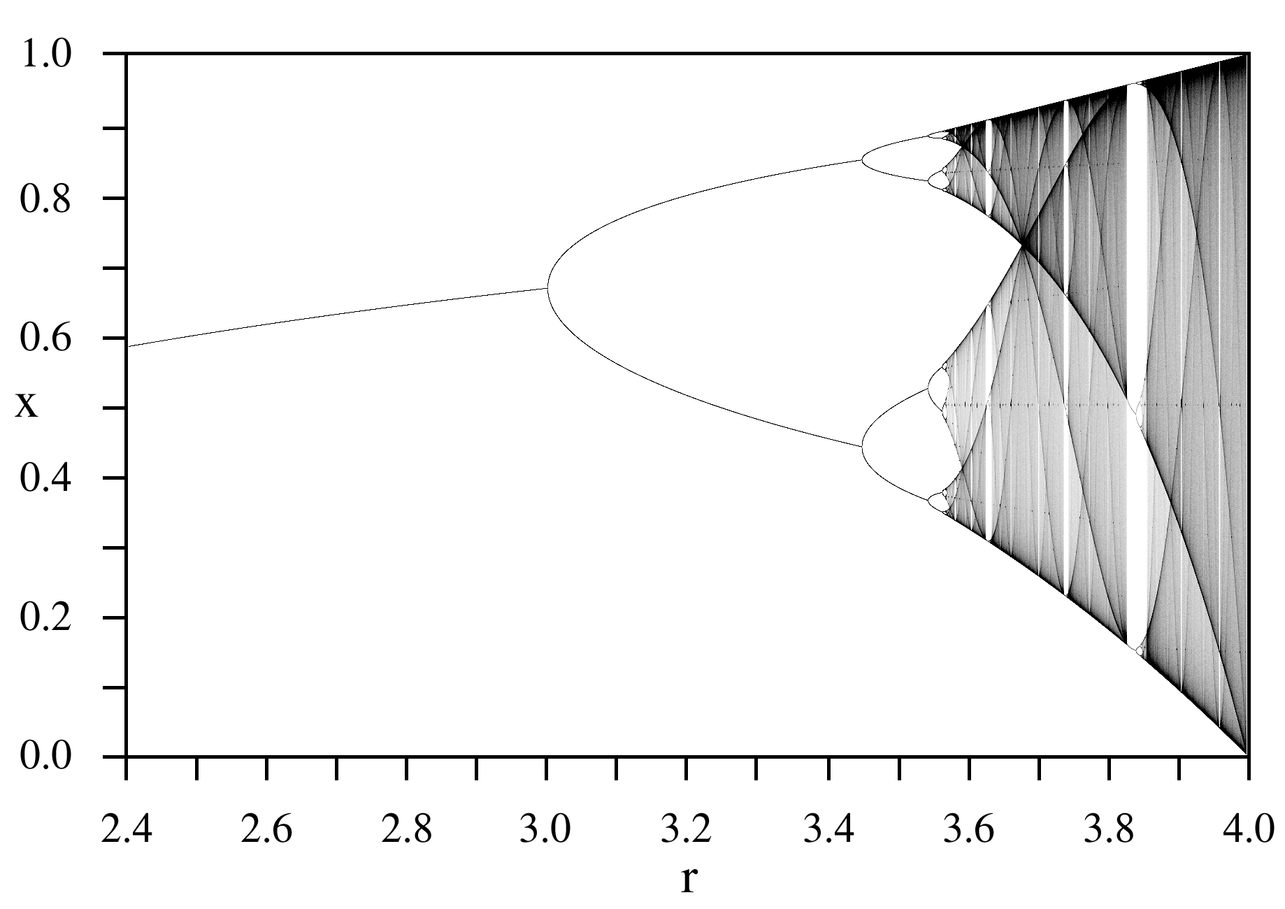
The bifurcation plot shows how a steady state changes as a parameter changes. Compute the long-term result of the logistic equation at the values of r = 2.9:0.001:4, and plot the steady state values for each $r$ as an r x steady_attractor scatter plot. You should get a very bizarrely awesome picture, the bifurcation graph of the logistic equation.

(Hint: Generate a single matrix for the attractor values, and use calc_attractor! on views of columns for calculating the output, or inline the calc_attractor! computation directly onto the matrix, or even give calc_attractor! an input for what column to modify.)

Part 3

Multithread your bifurcation graph generator by performing different steady state calcuations on different threads. Does your timing improve? Why? Be careful and check to make sure you have more than 1 thread!

Part 4

Multiprocess your bifurcation graph generator first by using pmap, and then by using @distributed. Does your timing improve? Why? Be careful to add processes before doing the distributed call.

(Note: You may need to change your implementation around to be allocating differently in order for it to be compatible with multiprocessing!)

Part 5

Which method is the fastest? Why?